International Journal on Computer Vision, Machine Learning, and Data Mining (CVMLDM)

1. Introduction

Butterflies are a member of the Lepidoptera order in insects family that represented by 1.5 million species in the animal kingdom. There are 170.000 butterfly species and they can be distinguishable from each other by wing shapes, textures and colours which vary over a wide range. Kayci reported that very similar species can be identified by examining the external structural features of the genital organs, particularly of the male [1]. Additionally, Paul and Ryan presented that also the identification of species can be done by molecular level studies [2]. Furthermore, Kaya et al. demonstrated that the butterfly species can be classified by using image processing techniques by a machine learning method with high accuracy [3]. In their study, the energy spatial Gabor filtered (GF) (different orientations and frequencies) images were used for representing images and classification was carried out by various classification methods. The highest obtained accuracy is 97% by ELM. In other studies, they obtained 96.3% and 92.85% classification accuracy, while employing grey-level co-occurrence matrix (GLCM) with multinomial logistic regression (MLR) [4], and GLCM with ANN [5] methods, respectively. Additionally we employed GLCM and local binary pattern (LBP) with ELM with 98.25%, 96.45% accuracy, respectively [6].

Although the obtained accuracies are high and the proposed methods can be acceptable because of low work and time requirements, Chaudhuri and Sarkar reported that the choice of proper texture analysis method is heightens the discriminative power [7] which is X is a major problem in image processing. Therefore the aim of this study is to investigate more proper texture analysis method for butterfly identification. The texture methods were reviewed in [8, 9]. Basically the popular ones are grey-level co-occurrence matrix (GLCM) [10], local binary patterns (LBP) [11], texture energy measure (TEM) [11, 12, 13], and each of them has a different characteristic and more effective for some types of problems, such as in GLCM, the statistical features are changed depending on selected angle and distance parameters. Especially, TEM has high ability to detect micro-patterns in image and it have been used for detecting edges, levels, waves, spots and ripples at chosen vector length neighbouring pixels in both horizontal and vertical direction since the butterfly species distinguish from each other by their morphological properties. TEM is based on filtering an image with predefined special masks and later their statistical features such as mean, standard deviation and entropy are used in place of images. TEM may have better performance than other alternative approaches. Because it provides several masked images from the original image that detects levels, edges, spots, waves and ripples in specified pixel neighbours and more useful features may be obtained from masked images [14], which is demonstrated by Pietikainen et al. [15, 16]. A considerable amount of literature has been published on TEM depend on its easy structure and high power of extracting distinguishable features such as bone analysis [13] in which 5-VL TEM masks were employed to analyse bone micro-architecture, ultrasonic liver images [17] and atherosclerotic carotid plaques [18]. Therefore, this study is aimed to evaluate and validate the applicability of texture energy measure method (TEM), which is defined by Law [12], for butterfly identification.

In this study, features were extracted by statistical variables from filtered butterfly images with 3, 5 and 7 vector length TEM masks. The relevant features were selected for decreasing the computational cost.  The proposed method is formed in two stages; first, texture features are obtained from a butterfly image by different sized TEM filters and second, the classification process with machine learning methods such as a k nearest neighbour (kNN), support vector machines (SVM), and extreme learning machine (ELM) were performed using these features. In this study, we wished to demonstrate that the texture features of organisms are also decisive among the external morphological features used in identification. The rest of the paper was organized as follows. The material used in this study was explained in the next section. In Section 3, the process of Law’s texture energy measures method was explained. Additionally, the concept of kNN, SVM and ELM machine learning methods and the proposed model is briefly described. Results and discussions are provided in Section 4, while Section 5 concludes the paper.

2. Material

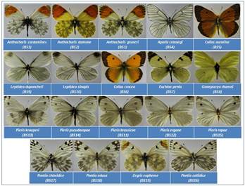
Specimens of butterfly species were collected in the Lake Van basin between May 2005 and August 2010 at altitudes of 1800 and 3200 m. [3-6], classified and imaged by the third author. The identification of butterflies were depending on the  morphological features of the extremities and organs on the head and thorax, textures and colours on the upper and lower sides of the wings as the methods explained by Carbonell [19], Skala [20], Hesselbarth et al. [21] and Tolman (1997) [22]. The image dataset was consisted of 10 images, for each of the 19 species and a sample of the dataset is shown in Figure 1.

3. Method

A variety of methods are used to assess butterfly textures. Each has its advantages and drawbacks, such as the energy spatial Gabor filtered [3], grey-level co-occurrence matrix [4], and local binary pattern [6]. Kaya et al. pointed out that the butterflies can be distinguished according to their textures [3-6], and TEM method is an effective method for detecting texture [15, 16]. In this study, TEM was used for extracting features. The TEM approach has a number of attractive features for detecting special texture types from an image, which will be described.

3.1. Texture Energy Measure

In TEM, firstly the image is filtered with predefined masks, which are formed with 1-D TEM vectors. These 1-D TEM vectors are defined for detecting levels, edges, ripples and spots in an image. There are 3 types of 1(one) dimension TEM vectors defined which have 3, 5 or 7 vector lengths (VL) [12, 13 and 23]. The VL shows in which range or neighbouring size the filters will detect. The 1-D TEM vectors are shown in Table 1.

Table 1. TEM Vectors.

	3 – VL	5 – VL	7 – VL
Level	L3=[1 2 1]	L5 = [1 4 6 4 1]	L7=[1 6 15 20 15 6 1]
Edge	E3=[-1 0 1]	E5 = [-1 -2 0 3 1]	E7=[-1 -4 -5 0 5 4 1]
Spot	S3=[-1 2 -1]	S5 = [-1 0 2 0 -1]	S7=[-1 -2 1 4 1 -2 -1]
Wave		W5 =[-1 2 0 -2 1]
Ripple		R5 = [1 -4 6 -4 1]

where [1];

• Level:  average grey level,
• Edge: extract edge features,
• Spot: extract spots,
• Wave: extract wave features,
• Ripple: extract ripples.

Each 1D TEM vector has its own structure and the characteristics of them is special to determine the same type of texture in the image. These 1-D TEM vectors determined and named as shown in Table 2.

For 3 and 7 VL only 9 TEM masks and for 5 VL, 25 TEM filters was defined and each filter has its own special property as seen in Table 2. The statistical features, such as; mean, standard deviation, entropy, skewness and kurtosis of filtered images are used for describing the images [13], since Tamura et al. reported that human texture perception is sensitive to first and second-order statistics and does  not  respond  to higher than  second-order [24]. Also, if the directionality of images isn’t important, then the mean of the horizontal and vertical vectors of the same filters can be used, for feature reduction; [23], such as

Table 2. TEM Filter Examples.

Mask	Calculation	Description
E3S3	E3T*S3	Edge detection in horizontal direction and spot detection in vertical direction  of 3 neighbouring pixels in both horizontal and vertical direction
W5W5	W5T *W5	Wave detection in both horizontal and vertical direction of 5 neighbouring pixels in both horizontal and vertical direction
L5R5	L5T *R5	Ripple detection in horizontal and grey level intensity in vertical direction of 5 neighbouring pixels in both horizontal and vertical direction
L7S7	L7T*S7	Spot detection in horizontal direction and grey level intensity in vertical direction  of 7 neighbouring pixels in both horizontal and vertical direction

3.2. Machine Learning Methods

k Nearest Neighbours (kNN) method is a popular and there are many versions of kNN methods such as nearest neighbour, weighted nearest neighbour and k nearest neighbour mean classifier.  This method depends on a simple idea, which is an unclassified data has the same class with its nearest neighbours. The kNN is optimized by determining the best suitable number of neighbours (k) and distance calculation method for computing the distance between the query and train data such as Euclidian, Manhattan and Supreme [25]. 

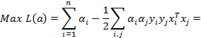
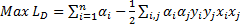
Support Vector Machine (SVM) algorithm tries to find one or multiple hyper-planes that separate point sets binding two or more conditions or events. An infinite-dimensional hyper-plane is differentiating a data set as one of the states on the one side of the plane and other states on the other side of the plane. The most appropriate plane is the one farthest from any neighbour points belong to a class.  In general, since a finite-dimensional data set cannot be decomposed linearly, the decomposition is achieved by transferring the data to a larger dimensional space. The most suitable hyper-plane, according to the support vector is the one which provides the widest separation between two classes. If there is such a hyper-plane it is the maximum-margin hyper-plane and this is called a maximal margin SVM classifier. For a linear separable condition SVM the decision function is expressed as follows [26],

where  are Lagrange factors obtained by the solution of the following convex quadratic programming (QP) problem [27].

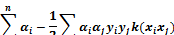
where; , . In classification problems which cannot be separated linearly, using smoothed margins for a minimum classification error in 1995, Cortes and Vapnik modified the detection of the maximum margin [28]. The modified decision function and the quadratic form of the dual problem are as follows [29],

where; ,  and the kernel is expressed as . After transferring the data to high-dimensional space with a kernel function, then it can be separated with maximum margin linear classification method [30]. The commonly used kernels are linear, radial-based polynomial, and sigmoid kernel functions.

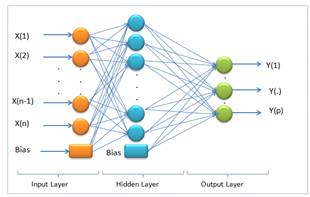
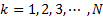
Extreme Learning Machine (ELM) is a training method for single hidden layer feed forward artificial neural networks (SLFN). The SLFN structure is illustrated in Figure 2.

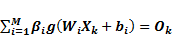
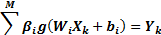
According to Figure 2, on determining that X(1⋯n) is input and Y(1⋯p) is output, the mathematical model with M hidden neurons can be defined as [31].

where W_(i1-in) and β_(i1-im) are the input and output weights; b_i is the threshold of the hidden neuron and O_k is the output of the network. g(.) denotes the activation function [32]. In a network of N training samples, the aim is with zero error ∑_(k=1)^N▒〖(O_k-Y_k )=0〗 or with min error ∑_(k=1)^N▒〖(O_k-Y_k )^2 〗. Therefore, equation 6 can be shown as below [33].

Because in the equation above  denotes output matrix in the hidden layer, equation 6 can be placed as [33];

where;

H denotes the hidden layer output matrix [31]. Input weights in ELM  and  hidden layer biases have been randomly produced, and the hidden layer output matrix H is obtained analytically. The procedure of training an SLFN is to seek the least-squares solution of the linear system  in ELM [34]:

Above,  is the smallest norm least-squares of  Furthermore,  indicates the Moore-Penrose generalized inverse of H. The norm of  is the smallest among all the least-squares solutions of [33-36].

3.3. Proposed Method

In this study, TEM and machine learning methods were used for butterfly species identification from 190 butterfly images, which were belonging to 19 species. The study consisted of 5 stages as seen in Figure 3.

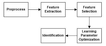
The process in Figure 3 can be summarized as follows briefly.

Block 1: RGB butterfly images were converted to grey images and resize to 512x512 pixel image to decrease the computational cost.

Block 2:  Getting statistical features, such as; the mean, standard deviation and entropy of filtered images.

Block 3: Ranking features with “Info Gain Attribute Eval” method in Weka for getting the worth of a feature by measuring the information gain with respect to the class [28].

Block 4: Optimization of kNN, SVM and ELM methods through butterfly data set.

Block 5: Classification of data set through kNN, SVM and ELM classification machine learning methods (decision stage).

4. Results and Discussion

4.1. Feature Extraction

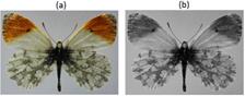
Firstly, to decrease the computational cost the images in the dataset were transformed from RGB to grey and a sample is shown in Figure 4.

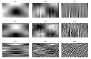
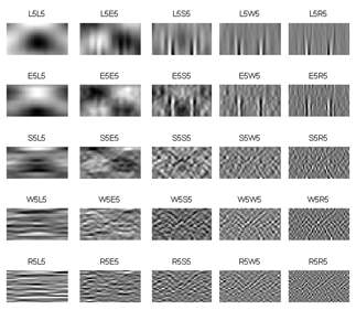
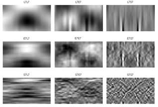
Secondly, the grey images are filtered by predefined TEM masks in each VL (3, 5 and 7). The filtered images (for the image in Figure 4-b), which are labelled by employed masks name, are shown in Figure 5, 6 and 7 for vector length 3, 5 and 7, respectively. The mean, standard deviation (STD) and entropy of the filtered images were used to describe the butterfly images. 27 features are extracted for 3 and 7 VL and 75 features for 5 VL extracted for each feature.

4.2. Feature Selection

The feature selection methods are used for determining the most relevant features in a dataset which may also consist of irrelevant, redundant or noisy features. Feature selection provides advantages like reduction of the computational cost, improvement of the data quality by means of filtering noisy features and enhancing the accuracy of machine learning method [37, 38]. In this study, the features were selected depend on “Info Gain Attribute Eval” method that evaluates the worth of an attribute by measuring the information gain with respect to the class, in Weka that is a collection of machine learning tools for data mining purposes including data pre-processing, feature selection, classification, clustering, association rules and visualization [39].  The most relevant three features extracted from 3, 5 and 7 VL TEM filtered images are shown in Table 3.

Table 3. The Feature Ranks of Statistical Variables from Vector Length 3 TEM Filters.

Vector Length	Feature Order	Mask Name	Statistical Feature
3 VL	1 2 3	L3T*E3 E3T*S3 L3T*S3	Std Std Std
5 VL	1 2 3	S5T*R5 L5T*W5 E5T*L5	Mean Mean Entropy
7 VL	1 2 3	L7T*L7 L7T*S7 L7 T*E7	Mean Std Std

Determining the best suitable number of features is done as follows. Firstly the features are sorted depending on their feature ranks and a new the dataset was generated with only the feature that has the highest rank and next the accuracy of using this dataset was calculated. The dataset was enlarged by adding the features one by one until it contained the whole dataset. Afterwards, the best dataset was determined by assessing the accuracy. The kNN method was used in this process. The obtained accuracies depend on the number of features are shown in Figure 8.

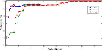
As it is clear from the Figure 8, the dataset was created by using the best 1^st-50^th feature obtained from 5 VL depends on the accuracies obtained with datasets. The accuracies of using a larger dataset did not increase and therefore the dataset was consisted of the 50 features that have the highest feature rank for decreasing computational cost without reducing accuracy. Further studies were done with this dataset.

4.3. Optimization of Machine Learning Methods

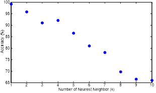
The kNN method was optimized by determining the best suitable number of nearest neighbours (k). The classification accuracies obtained by kNN while employed with different k numbers is shown in Figure 9.

The best suitable number of nearest neighbour is 1 for this dataset as it is clear in Figure 9. The butterfly is in the same species of its nearest neighbour and the accuracy of butterfly identification by kNN is decreased when the number of nearest neighbour is increased.

In this study, SVM optimization was done by choosing the best suitable kernel with kernel parameter. The accuracies obtained classification accuracies are sorted in Figure 10.

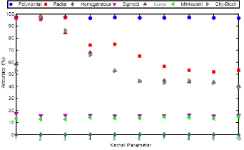
The best suitable kernel and parameter are; polynomial and 1, respectively as it can be observed from the Figure 10. The accuracy of using a polynomial kernel is stable.

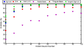
In ELM, number of neurons and the transfer function is determined by the accuracies obtained and they are illustrated in Figure 11.

The highest accuracy is obtained while employing SLFN, which has 60 Neurons in the hidden layer with tangent sigmoid transfer function depending on Figure 11. The accuracies of employing sigmoid, hard limit, triangular basis and tangent sigmoid transfer functions are nearly same while the SLFN has more than 50 neurons in the hidden layer.

4.4. Results of Classification

The obtained accuracies by classifying the selected features from the butterfly dataset with optimized kNN, SVM and ELM methods are sorted in table 4.

Table 4. The Error Depend on TEM Filter Vector Length.

Method	Accuracy (%)	STD
kNN	99.26	5.93E-5
SVM	98.16	6.98E-5
ELM	99.47	3.86E-5

The accuracy results obtained in this study are higher than the previous studies. It was 97%, 96.3%, 92.85%, 98.25% and 96.45% by employing GF+ELM [3], GLCM+MLR [4], GLCM+ANN [5], GLCM+ELM [6] and LBP+ELM [6], classification accuracies respectively. The classification accuracy obtained from ELM is slightly higher than the results obtained from kNN and was higher than SVM, which was suited to the results in [3, 6]. As a summary, the classification results were showing that the acceptable performance of TEM feature extracted butterfly identification method was not depended on machine learning methods. On the other hand, the performance of GLCM was depended on the employed machine learning method as seen the results of [4, 5, 6]. Therefore, the high performance can be seen as a result of using the TEM feature extraction method which suits the results of Pietikainen et al. [15, 16] study that compared Laws, co-occurrence contrast, and edge per unit area operators on Brodatz and geological terrain types and TEM performed better than other operators.

The authors strongly suggest that employing image processing methods are a better approach than using conventional diagnostic methods for identification. Since employing machine learning methods requires less effort and attention than time consuming and attention-seeking conventional diagnostic methods [6]. Additionally, image processing methods are cheaper than them. A huge image databases can be used for identification of each animal or plant, which may help the human development of caring them or learning a new approach from them. On the other hand, all images must be shot with an acceptable resolution; as Rachidi et al. demonstrated there is a strong relationship between image resolution and Laws’ masks texture parameters, such as when the pixel size was increased, the information contained in the images may be lost [13]. Therefore the images in the database must be in meaningful resolution.

5. Conclusion

The aim of the study is to identify butterfly species from their images instead of very complex, time consuming and expensive classical methods. For this reason TEM method, a texture analysis method was used for feature extraction. The main advantage of using TEM is; the TEM filters can detect edges, levels, waves, spots and ripples at chosen vector length neighbouring pixels in both horizontal and vertical direction. Since each butterfly species has a different colour or shapes, the TEM feature extraction method shows high performance of classification such as 99.26%, 98.16% and 99.47% by using kNN, SVM and ELM, respectively. Therefore, the results of this study were showed that the butterfly identification can be easily done by proposed machine vision method and the high performance of identification was not depending on the used machine learning algorithm, which was depend on used feature extraction method. These results show that the textures of butterflies may make an important contribution to the identification of butterfly species.  

References

[1] L. Kayci, “Erek Dağı (Van) Papilionoidea ve Hesperioidea Ekolojisi ve Faunası Üzerine Araştırmalar (Lepidoptera),” Priamus Suppl., vol. 6, pp. 1-47, 2007.
[2] P. Herbert and R. Gregory, “The Promise of DNA Barcoding for Taxonomy,” Syst. Biology, vol. 54, no. 5, pp. 852-859, Jul. 2005. View Article
[3] L. Kayci, Y. Kaya and T. Ramazan, “A Computer Vision System for the Automatic Identification of Butterfly Species via Gabor-Filter-Based Texture Features and Extreme Learning Machine: GF+ELM,” TEM J., vol. 2, no. 1, pp.13-20, Nov. 2013. View Article
[4] L. Kayci and Y. Kaya, “A Vision System for Automatic Identification of Butterfly Species Using a Grey-Level Co-Occurrence Matrix and Multinomial Logistic Regression,” Zoology in the Middle East, vol. 60, no. 1, pp. 57-64, Feb. 2014. View Article
[5] Y. Kaya and L. Kayci, “Application of Artificial Neural Network for Automatic Detection of Butterfly Species Using Color and Texture Features,” Visual Comput., vol. 30, no. 1, pp. 71-79, Jan. 2014. View Article
[6] Y. Kaya, L. Kaycı, R. Tekin, and Ö.F. Ertuğrul, “Evaluation of Texture Features for Automatic Detecting Butterfly Species Using Extreme Learning Machine,” J. of Experimental & Theoretical Artificial Intell., vol. 26, no. 2, pp. 267-281, Jan. 2014. View Article
[7] B.B. Chaudhuri and N. Sarkar, “Texture Segmentation Using Fractal Dimension,” IEEE Trans. on Pattern Anal. and Mach. Intell., vol. 17, no. 1, pp.72-77, Jan. 1995. View Article
[8] P. Maillard, “Comparing Texture Analysis Methods through Classification,” Photogrammetric Eng. & Remote Sensing, vol. 69, no. 4, pp. 357–367, Apr. 2003. View Article
[9] J. Malik, S. Belongie, T. Leung and J. Shi, “Contour and Texture Analysis for Image Segmentation,” Int. J. of Comput. Vision, vol. 43, no. 1, pp. 7–27, Jun. 2001. View Article
[10] R. M. Haralick, K. Shanmugam and J. Dinstein, “Textural Features for Image Classification,” IEEE Trans. Syst. Man Cybern., vol. 3, no. 6, pp. 610–621, Nov. 1973. View Article
[11] T. Ojala, M. Pietikäinen and T. Mäenpää, “Multiresolution Gray-Scale and Rotation Invariant Texture Classification with Local Binary Patterns,” IEEE Trans. on Pattern Anal. Mac. Intell., vol. 24, no. 7, pp. 971 – 987, Jul. 2002. View Article
[12] K. Laws, “Textured Image Segmentation,” Ph.D. dissertation, University of Southern California, LA, 1980. View Article
[13] M. Rachidi, C. Chappard, A. Marchadier, C. Gadois, E. Lespessailles and C.L. Benhamou, “Application of Laws’ Masks to Bone Texture Analysis: An Innovative Image Analysis Tool in Osteoporosis,” ISBI 2008, IEEE, pp.1191-1194, May 2008. View Article
[14] D-C Lee and T. Schenk, "Image Segmentation from Texture Measurement," Int. Archives of Photogrammetry and Remote Sensing, vol. 29, pp. 195-195, 1993. View Article
[15] M. Pietikaeinen, A. Rosenfeld, and L. S. Davis, “Texture Classification Using Averages of Local Pattern Matches,” in Comput. Sci. Center, University of Maryland, 1981. View Article
[16] M. Pietikainen, A. Rosenfeld, and L. S. Davis, "Experiments with Texture Classification Using Averages of Local Pattern Matches," Systems, Man and Cybernetics, vol. 13, no. 3, pp. 421-426, Jun. 1983. View Article
[17] C-M Wu, Y-C Chen and K-S Hsieh, “Texture Features for Classification of Ultrasonic Liver Images,” IEEE Trans. on Medical Imaging, vol. 11, no. 2, pp. 141-152, Jun. 1992. View Article
[18] C. I. Christodoulou, C. S. Pattichis, M. Pantziaris and A. Nicolaides , “Texture-Based Classification of Atherosclerotic Carotid Plaques,” IEEE Trans. on Medical Imaging, vol. 22, no. 7, pp. 902-912, Jul. 2003. View Article
[19] F. Carbonell, “Contribution a la Connaissance du Genre Agrodiaetus Hübner (1822), Position Taxinomique d'Agrodiaetus Anticarmon Koçak, 1983 (Lepidoptera, Lycaenidae),” Linneana Belgica, vol. 16, no. 7, pp. 263-265, 1998.
[20] P. Skala, “New Taxa of the Genus Hyponephele MUSCHAMP, 1915 from Iran and Turkey (Lepidoptera, Nymphalidae),” Linneana Belgica, vol. 19, no. 1, pp. 41-50, 2003.
[21] G. Hesselbarth, H. V. Oorschot, and S. Wagener, “Die Tagfalter der Türkei,” Bochum, 1993.
[22] T. Tolman, “Butterflies of Britain and Europe,” London: Harper Collins Publishers, 1997, pp. 320. View Book
[23] G. Lemaitre and M. Rodojevic “Texture Segmentation: Co-occurrence Matrix and Laws’ Texture Masks Methods,” pp. 1-34. View Article
[24] R. Tamura, S. Mori, and T. Yamawaki, “Textural Features Corresponding to Visual Perception,” IEEE Trans. SMC, vol. 8, no. 1, pp. 460-473, Jun. 1978. View Article
[25] “kn-Nearest Neighbor Classification,” IEEE Trans. on Inform. Theory, vol. 18, no. 5, pp. 627-630, Sep. 1972.
[26] J. Park, “Uncertainty and Sensitivity Analysis in Support Vector Machines: Robust Optimization and Uncertain Programming Approaches,” University Of Oklahoma, 2006. View Book
[27] V. Kecman, “Learning and Soft Computing: Support Vector Machines, Neural Networks, and Fuzzy Logic Models,” Cambridge: MIT Press, 2001. View Book
[28] C. Cortes and V. Vapnik, “Support-vector Networks,” Mach. Learning, vol. 20, no. 3, pp. 273-297, 1995. View Article
[29] B. Kepenekçi and G.B. Akar, “Face Classification with Support Vector Machine,” in IEEE 12th Signal Process. and Commun. Appl. Conf., pp. 583-586, 2004. View Article
[30] T. Joachims, “Learning to Classify Text Using Support Vector Machines: Methods, Theory and Algorithms,” London: Kluwer Academic Publishers, 2002. View Book
[31] S. Suresh, S. Saraswathi, and N. Sundararajan, “Performance Enhancement of Extreme Learning Machine for Multi-category Sparse Data Classification Problems,” Eng. Appl. of Artificial Intell., vol. 23, no. 7, pp. 1149-1157, Oct. 2010. View Article
[32] R. Hai-Jun, O. Yew-Soon, T. Ah-Hwee, and Z. Zhu, “A Fast Pruned-extreme Learning Machine for Classification Problem,” Neurocomputing, vol. 72, no. 1-3, pp. 359-366, Dec. 2008. View Article
[33] G.B. Huang, Q.Y. Zhu, and C.K. Siew, “Extreme Learning Machine: Theory and Applications,” Neurocomputing, vol. 70, no. 1-3, pp. 489-501, Dec. 2006. View Article
[34] Q. Yuan, Z. Weidong, L. Shufang, and C. Dongmei, “Epileptic EEG Classification Based on Extreme Learning Machine and Nonlinear Features,” Epilepsy Res., vol. 96, no. 1-2, pp. 29-36, Sep. 2011. View Article
[35] S. D. Handoko, K. C. Keong, Y. S. Ong, G.L. Zhang, and V. Brusic, “Extreme Learning Machine for Predicting HLA-peptide Binding,” Lecture Notes in Comput. Sci., vol. 3973, pp. 716–721, 2006. View Article
[36] W. Zong and G. B. Huang, “Face Recognition Based on Extreme Learning Machine,” Neurocomputing, vol. 74, no. 16, pp. 2541–2551, Sep. 2011. View Article
[37] I. Guyon and A. Elisseeff, “An Introduction to Variable and Feature Selection,” J. of Mach. Learning Res., vol. 3, pp. 1157-1182, Jan. 2003. View Article
[38] M. Dash and H. Liu, “Feature Selection for Classification,” Intell. Data Anal., vol. 1, no. 3, pp. 131–156, 1997. View Article
[39] H. Witten and E. Frank, “Data Mining: Practical Machine Learning Tools and Techniques,” 2nd Edition, San Francisco, Morgan Kaufmann, pp. 420-3, 2005. View Book